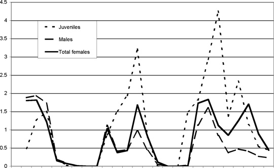
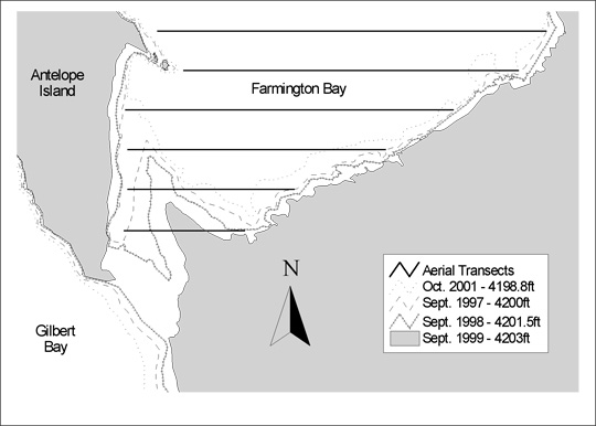
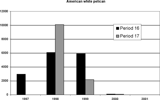
Discussion

Habitat Changes with Lake Elevation Shift

It is important to consider the GSL elevation during the five-year study in context of historical lake elevation because of the known dramatic change in lake and shoreline habitats that occur due to the flat bottom nature of this playa lake. During the study period, the lake ranged within 25% of the 20.5' range known to occur over the 154-year lake elevation record period (Table 3). The five-year elevation pattern mimicked a period spanning 20 years, from 1910-1930. We consider the study period of 1997-2001 to be a reasonable representation of typical water level patterns, though condensed into a shorter time frame. The average GSL elevation data and its deviation from the average reflect the long-term tendency of the lake to return to an equilibrium around 4200' ASL (Arnow 1980). At the same time, a few inches of gain or loss of lake elevation can have an exceptional effect on GSL shoreline habitats. Shoreline fluctuation during the five-year study affected lake habitats in ways similar to those observed in the past. When the lake was at 4204.6' ASL, it flooded emergent vegetation stands in the same locations and reduced the shoreline playa reach between the water edge and uplands at other locations. Species that use flooded emergents for nesting colonized in several locations around the lake. At this lake elevation, some mud bars were covered, including some that were used by colonial nesters at other times. Land bridges between the mainland and small islands were covered by water, enhancing the attractiveness of the islands for colonial nesting species. Also, the distance between nearby uplands and water was shortened and water lapped at the feet of dikes and levies. In some cases, there was salt water intrusion into WMA ponds. Of note was the flooding of substantial bars that, at lower elevations, extrude for miles into parts of the lake. This was especially true in Farmington Bay where the bar south of the Great Salt Lake Shorelands Preserve was inundated, as well as the bar at the northwest end of the Jordan River Delta complex.

An antithetical condition occurred in 2001 and also to some degree in 1997 when the lake dropped below 4200'. The shorelines were dominated by extensive open mud bars, which in some cases isolated emergent wetlands from the salt water. The interface between salt water and fresh water wetlands and uplands was widened in many places by hundreds of meters. Colonial nesting species, especially gulls, occupied low relief mud bars and other islands. Nesters abandoned these nesting sites as land bridges became exposed and accessible to predators. Emergent wetlands were salt burned and set back to early serial stages, and mosaic patterns of new emergents were established. Distance increased between shoreline foraging habitat and other lake habitats like fresh water inflows.

Changes in lake volume affect lake limnology, as an artifact of lake elevation. During low lake periods, the decreased volume increases brine concentration and subsequently influences obligate halophytes and halophiles occurring at GSL. In general, lower brine concentrations foster greater species diversity, but may decrease productivity of individual species. High concentrations within a certain range (120-170 ppt) often generate lower species diversity, but large numbers of the species are present. These conditions occurred at GSL during the study period with excellent brine shrimp and brine fly populations during the years of 1997, 2000, and 2001; in these years, the Gilbert Bay portion of the South Arm was below 4202'ASL during mid-summer and early fall (Figure 7).

Figure 7. Brine shrimp numbers per liter in the South Arm, Great Salt Lake, 1999-2001.

In addition to lake elevation, there are other factors that affect lake limnology. Seasonal ambient and water temperatures are important, and nutrient recharge may affect lake production and species compositions of algae and invertebrates. A major breach in the Union Pacific railroad causeway near Lakeside, between Gunnison and Gilbert Bays was improved between the 2000 and 2001 survey years and allows better water flow exchange.

Changes in limnology in turn affect fisheries at GSL. During 1997, 1998, and 1999 a fishery occurred in the Bear River Bay/Willard Spur region. This fishery spanned from approximately two miles north of the Great Salt Lake Minerals Company (formerly IMC Kalium) culvert to the Bear River National Wildlife Refuge, and east in Willard Spur to the Willard Bay dike. Large numbers of several species of piscivorous birds consumed carp and gizzard shad during these years. In mid-summer 2000 and extending through 2001 this fishery was lost due to reduced flows from the Bear River and falling lake elevations that left mud flats and very shallow water as this region dried up.

Weather Variances

On several occasions during the mid 1970s, extreme wind events over the GSL drove Wilson’s and red-necked phalaropes off the lake. On one occasion, large flocks of phalaropes were carried over the UDWR Northern Region office by wind from the southwest. As the wind subsided these flocks were observed returning west to the lake from the Ogden area. On another occasion a person brought several Wilson’s phalaropes into the UDWR Northern Region office that had been found dead on Willard Peak. After an interview, it was learned that the phalaropes had been picked up by a southwest wind and carried to the Willard Basin where a severe rainstorm changed to hail at higher elevations. This storm had killed large numbers of the species in the Willard Basin area. With this information, D. Paul drove to the basin where he observed several hundred dead Wilson’s phalaropes in an area of several square kilometers.

Although extreme conditions similar to this unique event were not recorded, there were episodes of high wind, cold periods (Spring 1999), and long, dry periods (July 2000-2001). Each of these conditions had an effect on habitat, bird distribution and surveyor capacity.

Evaluation of Methods

Most missing data points were sporadic, and filled in by taking an average of the numbers on either side of the gap. However, when two or more consecutive missed points occurred, the gaps were not filled. These holes in the data set do affect total counts at the all-lake level, but especially at the level of survey area. In large part the data reported are in the format of a five-year mean, and the missed counts are tempered by averaging. Comparisons between years are not as reliable because of missed surveys in areas. In some cases areas were not surveyed at all for a particular year. To make direct year-to-year comparisons, it is necessary to select areas that are similar in the extent of their coverage and then draw conclusions for those areas only, not from the entire GSL ecosystem. The Survey Area Descriptions section (Appendix 4) details the degree of coverage by survey area for the study period.

Detection rates were variable across survey areas. Most often shoreline areas were classified as having 100% detection. The wetland complex areas with tall, emergent vegetation, long viewing distances or access difficulties did not always have good detection rates. These situations were fairly consistent throughout the five years, and therefore the counts were constant in the portions of an area that had clear viewing. These counts are still valuable and may be able to indicate changes within an area. For this reason and others the project managers believe that the numbers reported in this document are sound, but conservative.

Several survey areas were not covered for the entire five-year study period. Some areas were surveyed intermittently while others were covered for the first or last years of the study (Table 2). Incomplete survey area data were rolled into an analysis of the years for which they were surveyed but excluded from any between year analyses.

Some survey sites are missing surveys from over the course of the five-year study. Most surveys missed were only intermittent with the surveys just before and after the missed survey period in place. In this circumstance, counts before and after the gap were averaged to estimate the missing data point.

Most survey forms were complete when turned in, especially for total count data. When information was missing, contacts with the survey team leader or surveyor were generally sufficient to make the data complete. The most incomplete or confusing data from the field crews pertained to point sample data. The survey form was not user-friendly, and the complexity of recording habitat type estimates by percent within the point and bird use within the types was the most difficult task requested of surveyors. Even so, with some effort on the part of the data manager, most of the sample point data was entered and used.

When GSL open water transects were developed in 1997, the GSL elevation was 4201.6’ ASL (June 15, 1997). The transects for the open water in Farmington, Ogden, and Bear River bays were established so that the end points occurred one half mile off shoreline. Shoreline survey protocols required observers to count birds within a half-mile window, one-quarter mile on each side of the survey line, which paralleled the shoreline 91 meters (100 yards) from the water’s edge. Thus, a surveyor counted birds out to 275 meters, or nearly 1⁄4 mile, therefore reducing the bias of double counting birds observed in the aerial survey. However, because the shoreline fluctuated with changing lake elevations in neighboring survey areas there were potential overlaps between aerial and shoreline surveys. The 1997 aerial transect endpoints were used throughout the five years of study, but the potential overlaps occurred when the GSL elevation fell below 4201.6’ ASL for two reasons. First, when the lake was down the aerial survey transect endpoints were within the adjacent shoreline survey areas as the surveyors on foot moved out with the GSL shoreline to maintain a 91 m travel lane from the water’s edge. Second, when two sandbars extruded into the aerial transects, they dramatically re-configured the shoreline travel route (Figure 8). However, these overlap issues were addressed reducing the potential double count bias. The conflict with the dynamic shoreline was resolved in most cases through the aerial coverage. Bird counts were stopped short when the transect was within an estimated 1⁄2 mile of the shoreline. This was really only an issue in 2001 when the GSL was considerably lower than 4201’ ASL, and in some late summer survey periods when the water level was down. Most of the extruding sandbar problems were resolved through communicating between aerial and ground surveyors.

As outlined in the Methods section of this report, a moving sample point was developed so that the inventory of birds using the shoreline was constant through the five-year study. This floating point occurred 91.44 m (100 yards) from the shoreline and at right angles between the original point sample marker and the GSL shoreline. This condition was largely achieved during the study. Exceptions occurred only if original point sample markers were lost during the winter or needed replacement. We used GPS references for replacement whenever possible, but the need to replace a marker was rare, because salt water retarded surface freezing during winter months.

We identified one set of circumstances that biased the comparison of bird use and habitat types at individual point sample sites. As surveyors moved out or back from point sample markers with shoreline fluctuations, they often moved into different habitat types or closer to or farther from specific habitats and landscape features. In some years, observers were hundreds of meters from the point sample marker of 1997. Therefore, perhaps the best comparison of data between years within point sample areas is for the data of birds directly associated with the actual shoreline.

The study managers did work to reduce bias from individual surveyor capacity to estimate distances accurately, especially at a quarter mile (440 yards or 402.3 m). We held an annual field day each spring for Waterbird Survey Team Members, and part of the training was spent helping surveyors develop distance estimation skills. Several tools were provided including the use of auxiliary posts placed at 440 yards on each side of a point sample marker to visually assess ½ mile diameter sampling areas. We know there will be variation by surveyor in estimating the boundaries of the sample point sites, however, the same surveyors made most of the counts throughout a season and from year to year. Therefore, bias should be consistent.

Figure 8. Aerial transects and GSL shoreline configuration at high and low lake elevations.

Data describing behavior of waterbird suites by habitat type were collected at point sample locations. Pre and post survey season meetings were held to assist survey team members in the use of the sample point and other survey protocols. This behavioral data was used mostly as an index to the reason for bird presence in this report. It was collected as a sample of one point in time (one observation / bird) and, therefore, is only a field note pertaining to habitat use within the point sample for each sample period.

From the five-year data set and other information and observations at the GSL, it is obvious that we have missed peak occurrence periods for some species of waterbirds. This is especially true for waterfowl and a few other species. Notably missing are: bufflehead, canvasback, common goldeneye, northern shoveler, northern pintail, mallard, redhead, western grebe, scaup, and larger numbers of eared grebes. There are some waterbird species that are present in large numbers outside of this study period. Tundra swan, snow goose, greater and lesser scaup, some sea ducks, common merganser, Bonaparte’s gull, and a few species of northern gulls are the majority of these birds missed by the survey. These are the primary components of frame bias associated with the data set. Beyond missing the peak period for some species, there were other species that occurred in large numbers at the lake, but often not within the survey areas. These include Wilson’s phalaropes and red-necked phalaropes that occupy open regions of the GSL not in a survey area. Other species such as bitterns and rails were secretive and often not detected. Species like long-billed curlews and willets use uplands for nesting and part of their populations were not successfully surveyed.

The database that was established at the beginning of the Waterbird Survey was not an effective tool for several reasons. First, the format of the database underwent some changes between 1997 and 1998 especially within the point sample section, making data from 1997 difficult to use and incomparable with the other years. Second, the data entry system was not user friendly. The screen for actual data input was different from the screen to view all data, and as a result quality control during the data entry process was cumbersome. The database was quite complicated with different people responsible for entering data during each of the five years of study. Data querying and extraction from the database were also difficult, as data managers were not trained in the use of the program. Third, the Waterbird Survey data set was meant to be shared with others within and without the Utah Division of Wildlife Resources, but because the selected program is not universally used, requested data had to be transferred to a spreadsheet to make it functional, therefore, the tables of GSL Waterbird Survey data produced by Jonathan Bart USGS were utilized almost exclusively in the analysis of this data set.

The GSL Waterbird Survey data set is extensive, and the contents of this report only begin to answer a few of the many questions that may be addressed. This report does, however, provide good descriptions of bird use at GSL by species, by time period, and by survey area. Only basic statistical analyses have been completed to this point; a more sophisticated statistical analysis may be appropriate in drawing out additional detailed patterns of habitat selection and population fluctuations that may exist. Project managers have made great efforts to produce a database that is solid and broad in its reach of area, time and species coverage. This has been achieved and is a good foundation for further investigations of waterbird use of the Great Salt Lake ecosystem.

Survey Coverage

It was difficult to maintain consistent coverage over the five years, as we were dependent upon volunteer help. Also, natural barriers to optimal viewing compromised the quality of coverage in some areas. In a separate document, the greater Great Salt Lake area is evaluated as to the extent of appropriate shorebird habitat, detection rates around the lake are described, and suggestions are given for methods to provide for complete coverage. This document is titled “A Plan for Monitoring Shorebirds During the Non-breeding Season in Shorebird Monitoring Region Utah-BCR 9 (Great Basin)” and focuses on shorebird species. However, similar principles apply to other waterbird species and the evaluation could be expanded to include other species as needed (Manning et al. 2002). It is included as Appendix 7 at the end of this report.

Migration Chronology

A primary target of the five-year study was to capture the pulse of waterbirds as they move into, out of, and within the GSL ecosystem. We know from the high lake years of the 1980s that species move between systems in the intermountain region and beyond as local conditions change. The white-faced ibis is an example. In the mid 1980s, the GSL inundated much of the historical nest site habitat and subsequently ibises exploited improving water conditions elsewhere in the west. Oregon, Idaho, Nevada and northern Utah wetlands experienced expanding breeding populations of ibises. After the flood years and as habitat conditions improved for ibises they again colonized re-established emergent wetland vegetation sites at GSL. This study refines the current understanding of how waterbirds like white-faced ibises use the GSL ecosystem through the season.

In the evaluation of methods, frame bias was discussed for species that are on the margins of time pertaining to the study period. These species fit within six categories that we identified as periods of use in the migration chronology of waterbirds claiming some time and space at GSL (Table 6). These six periods are (1) April, departing winter residents; (2) April-May, migrants to breeding grounds; (3) April-September, local breeders; (4) July-August, early migrants to wintering grounds; (5) August-September, late migrants to wintering grounds; and (6) September, arriving winter residents. These categories are not mutually exclusive, and there are many species that fall into several of the descriptions. The degree to which species are present at GSL is well documented by this study. A good example of species presence through several periods is the American avocet. Avocets arrive from their wintering grounds on the west coast of Mexico in late March and by late April, approximately half of the peak GSL population is present and begin to pair up and establish nesting colonies. Some 60,000 to 100,000 breeding adults are present into April. Their young and arriving migratory individuals begin to flock and gorge on September brine flies. At the peak population size of 200,000 to 300,000 avocets depart GSL in late September and October.

For most departing winter residents (Migration Chronology Period 1), April is the end of their winter residency at the GSL. Winter residents return near the end of the survey season (September/October). The migrants to breeding grounds in Period 2 will stay at GSL to breed or travel farther north. Some individuals of these species associated with nesting at GSL (e.g., willets, move through the lake to nest at the northern extension of their range. Others still have many hundreds or thousands of miles to travel (e.g., long-billed dowitcher, black-bellied plover, greater yellowlegs, red-necked phalarope). There are at least 28 species that utilize the GSL ecosystem for breeding. There are some species that leave for their wintering grounds from the GSL in July and August. These include most of the peeps, many black-necked stilts, California gulls, Franklin’s gulls, greater yellowlegs, lesser yellowlegs, marbled godwits, white-faced ibises, willets, and Wilson’s phalaropes. Some of these species have been at the GSL though most of the survey periods, but others are just coming through from sites further north. This is also the case for species in the late migrants (August-September) category. In this group, there are many waterfowl species that are just arriving to GSL. Some continue on, while some stay until ice-up. Others, like the eared grebe, use GSL as a molt migration site. The ring-billed gull sometimes stay the winter, and other times passes through. The GSL breeding populations and their offspring are augmented by migratory populations of the same species in later survey periods. This seems to be true of avocets and pelicans for example.

The assessment of bird use days at GSL indicates that the greatest period of use begins halfway into the survey season and lasts through the remainder. Because of the numerical make up of occurrence, the waterfowl category is of great magnitude. It is suspected that bird use days remain strong well into the fall, beyond our periods of survey. Another important period of use is concurrent with summer and late fall halophile production of brine flies and shrimp.

The migration chronology data also demonstrate the dynamics of spring as birds move through the ecosystem. This is especially true for long-range migrants. Western sandpipers can occur in thousands at the lake in some survey sites, and dissipate before the next 10-day survey block. Red-necked phalaropes, Wilson’s phalaropes, and eared grebes are similar in this regard, as they pass through to breeding grounds.

Species Distribution

Shorebirds

The distribution of shorebirds at GSL varied by species. There were even some changes in habitat type use by the same species during different times of the survey season, and some that keyed on the same geographic locations despite changes in lake elevation. The magnitude of occurrence of some long-range migrants seemed to change between spring arrival and fall passage. These observations are made by examining five-year averages by survey period for each survey area. There is some variation to these mean numbers if each survey year is examined separately. However, these variations in distribution are more contingent on survey site than survey period. For some years the habitat type is different for the same survey area as a consequence of lake elevation and transitory shoreline, or the availability of water to manage wetland complexes. At other times wetland managers adjusted water levels as part of a prescribed application.

Following are some highlights of shorebird presence on the lake through the survey season. These comments are based on data presented in Appendix 6. For details of occurrence by location see Survey Area Descriptions (Appendix 4).

American avocets and black-necked stilts both seem to use managed wetland complexes extensively from April-July. Starting in August a preponderance of avocets disperse to GSL shorelines and congregate in large numbers in Farmington Bay. This is true too for black-necked stilts, but they also use east Gilbert Bay and Bear River Bay in large numbers.

Long-billed dowitchers and greater and lesser yellowlegs prefer to use wetlands with pools and ponds bordered with emergent vegetation. In April, and May, and July through September, dowitchers are found in large numbers at Bear River MBR and Farmington Bay WMA complexes, and can also be found in small concentrations throughout GSL wetland complexes. The two yellowlegs species are often observed together from April into early May, and again in late June through September. The largest numbers occur in Farmington Bay WMA, Ogden Bay WMA, and Bear River MBR.

Marbled godwits occur at the lake in mid April, on their return to the prairies for breeding. In the spring, the largest numbers were recorded at Bear River MBR and Ogden Bay WMA. Late June through September, they are present in the tens of thousands within the Bear River Bay complex, especially in the Willard Spur.

From April through mid September, snowy plovers are found in numerous playas and shoreline reaches. Large numbers were located in the Locomotive Springs WMA and Salt Wells Flat WHA. They were also present in good numbers at Stansbury beach and along the South Shore, within the Inland Sea Shorebird Reserve, along the Audubon beach, and in the Harold Crane WMA complex.

Wilson’s phalaropes appear at the lake in open water and associated wetlands during two concentration periods. First, in late April and early May they locate at Bear River MBR, east Gilbert Bay and Farmington Bay for a stop along their spring migration northward. Second, they return from breeding grounds in the intermountain west and prairies in June, build into July when they congregate in large flocks around Bear River MBR, the shorelines of the lake, and especially on open water reaches of GSL. Large flocks were counted in Gilbert Bay both in and out of Waterbird Survey areas, and also in Farmington Bay, and the largest flocks occurred around Carrington Island, along the Magcorp dike, and on the west shore.

Black-bellied plovers arrive in spring and again in late summer when they are observed in small flocks. The largest groups are consistently observed along the southern end of Antelope Island and the shoreline south of the Crystal Marsh and west of the Audubon properties. In some years, other sites of concentration are the Howard Slough shoreline and Ogden Bay WMA.

Least sandpipers are present in April and May and most commonly observed on the South Shore, Stansbury beach, the Inland Sea Shorebird Reserve, Farmington Bay WMA, and Bear River MBR. They return in August, locating again at the south end of the lake, Farmington Bay WMA, Inland Sea Shorebird Reserve and the Magcorp dike.

Western sandpipers arrive in late June and are seen though August. Some counts exceeded 150,000 individuals at Bear River MBR. Large numbers were also observed at Ogden Bay WMA, Farmington Bay WMA, the South Shore including Stansbury beach and the southeast shore of Antelope Island.

Sanderlings often occupy strips of sandy beach around the South Shore and along gravel dikes and causeway road structures including the Antelope Island State Park causeway, Magcorp dike, and dikes at Locomotive Springs. They are present at GSL April through May.

Colonial Waterbirds

Due to the close proximity of nesting colonies to some survey areas colonial waterbird distribution observations and population estimates within the ecosystem may be biased for some nesting species. In fact, several survey areas had colonies within their boundaries. This was true for California gulls, American avocets, black-crowned night herons, black-necked stilts, Caspian terns, eared grebes, Forster’s terns, Franklin’s gulls, western grebes, snowy egrets, and white-faced ibises. Some of these species do not always nest in dense colonies (e.g., American avocets and black-necked stilts), but most others do. The survey only required observers to report nesting activity during collection of point sample data. American white pelicans are an important species where no nesting activity took place in a survey area. The only nesting colony occurs on Gunnison Island, 35 miles from the nearest survey area.

Many waders are piscivorous species and were normally observed in parts of the ecosystem where fisheries occur. This was also the case for western grebes, Clark’s grebes, double-crested cormorants, Forster’s terns, Caspian terns, and black terns, all fish by diving into and under the water surface. These foraging conditions occurred at various locations around the lake and were largely associated with the three major river deltas of the Bear, Ogden/Weber, and Jordan. Occurrence was also noted at the mouths of smaller tributaries, canals and other artificial structures. Bear River Bay and Willard Spur portions of GSL held a fishery through the first three and a half survey seasons. The carp and gizzard shad fishery deteriorated with the hot, dry summer of 2000 continuing into 2001 when the Willard Spur was almost completely dry. Large carp carcasses were visible from the air in shallow water and on mudflats in the Bear River Bay region outside the D-line dike of Bear River MBR in mid summer 2000 and beyond. This affected fish-eating species distribution due to lack of a suitable fishery.

Observations of American white pelicans during the five-year study described how piscivorous species were influenced by variable conditions in GSL fisheries. Distributions of American white pelicans by survey period (Appendix 6) reflect specific site importance during an average year for pelicans. Areas of pelican concentration were the Bear River system and State WMAs on the east side of the lake. If the data are examined as annual means, counts of pelicans during late summer of 2000 and 2001 drop dramatically (Figure 9). These declines directly correlate with observed fishery loss in the Bear River system. Other fish eating waterbirds were also affected in a similar manner. However, the magnitude of effect depends on the species. Terns that forage on smaller fish, and grebes that dive, have some alternative fisheries in the area, such as Willard Bay Reservoir. Regardless, the quality of the fishery in the Bear River system has a profound affect on bird occurrence in the area.

The California gull is an example of a ubiquitous, breeding, colonial species at the GSL, with a broad diet and exploitative foraging behavior. Five-year mean counts by survey period show this species’ universal use of the GSL with some hot spots of occurrence near breeding colonies. These conditions are apparent in the months of June and July when the colonies are active with young (Appendix 6). In August and September, California gulls are found exploiting the large numbers of brine flies and brine shrimp in open water and shoreline areas.

White-faced ibises are a colonial species that establish colonies in emergent vegetation but spend much of their foraging in flood-irrigated agricultural lands feeding on earthworms and other invertebrates. Because the majority of their activity around the lake proper is associated with nesting, it is obvious where the nest sites occurred within wetland systems (see Appendix 6—White-faced Ibis Distribution by Survey Period, Periods 9 and 10).

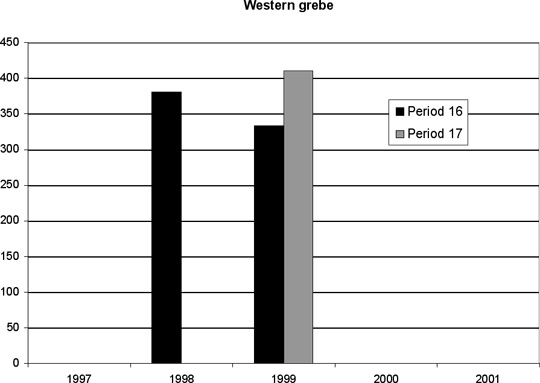
Figure 9. Numbers of American white pelicans and western grebes at Willard Spur (28)
during survey periods 16 and 17, 1997-2001. In 1997 survey work was not completed
during period 17. No western grebes were recorded in the Willard Spur during
survey periods 16 and 17 of 2000 and 2001 because the area was dry.

Waterfowl

The distribution of waterfowl at GSL wetlands is well understood-data have been amassed for well over a half-century-and data from the five-year study show those same patterns (Appendix 6). Ducks occur in large numbers during April (survey periods 1 and 2) as they pass through the area en route to breeding grounds. Then they start to re-appear in late June when some molt migration takes place, and build in numbers through September when the largest numbers of all ducks materialize, especially at the managed systems, Bear River, and Farmington bays.

These are but a few examples of the distribution of different species across the GSL ecosystem through the 17 survey periods. Examination of individual Species Accounts (Appendix 5) and specific Survey Area Descriptions (Appendix 4) allows for a more detailed understanding of how each species uses the GSL landscape during the months of April through September. To better understand how lake elevation affects species distribution, see also Species Distribution at High and Low Lake Elevations (1999 and 2001, respectively) in Appendix 8.

Breeding Species

These data are taken from all-lake five-year means for survey period nine (end of June, beginning of July), and are assumed to be the peak breeding time (Table 7). However, Waterbird Survey areas did not cover all of the GSL breeding grounds, and some species have peak numbers later in the season. California gulls breed on many islands outside the GSL Waterbird Survey study area and therefore this potential breeding adult figure would underestimate their actual numbers. American white pelicans also breed outside the survey area but because of their use of fresh water fisheries within the survey area, the population estimate from survey data should be more realistic. The actual five-year average of American white pelicans from the Gunnison Island breeding adult survey is 13,338 for 1997-2001, a difference of 3,440 from the WBS estimate. If the high year (1999) is dropped the four-year average is 12,183 or a difference of 2,285. These estimates might also be useful in assessing the percentage of the breeding adult population that forages outside the survey area (i.e., American Falls Reservoir, Idaho).

Species Accounts

Data reported by species are valuable in drawing conclusions about GSL populations as they relate to populations of a larger geographical area. It is interesting to note what percentage of North American, or worldwide, populations are found at GSL. Equally important is a review of the scale of a particular population. All species do not occur at the same magnitude. For example, the estimated number of mallard ducks in North America is close to 7.5 million, and the high count recorded at GSL is137,468. The GSL population is 2% of the continental population. The highest count of marbled godwits at GSL during this study was 43,833, less than one-third the number of mallards. However, the estimated population size for marbled godwits in North America is 171,500, of which the GSL group represents 25%.

Three numbers for waterbird species present at GSL are reported in the Species Accounts: mean, peak and high count. All are useful in describing waterbird use of the GSL ecosystem. The mean is a stable and conservative figure that indicates likely population sizes during the respective time frame of presence for each species in any given year. The peak number is the highest count for one survey period. This is a mean over five years and is graphically displayed. The high count is the greatest number recorded in one survey during the study. This value may represent a time of optimal conditions at GSL for a particular species, or it may be an artifact of other circumstances that affect a species during other parts of its life cycle.

Bird Use Days

The bird use day calculation is useful in considering numbers of birds present at GSL in conjunction with their length of stay. A bird day is defined as one bird spending 24 hours within the study area during the study period. On average, between April and September (170 days) waterbirds spend 86,752,258 bird days at GSL. This number alone illustrates the importance of GSL and its allied wetlands to many waterbird species. This presence includes a range of activities: migratory stopovers, breeding cycles, molt migrations and a portion of year round residency. It is a way to combine observations of species that migrate through the area in large flock sizes (phalaropes) with species that spend much of the year at GSL (gulls), and species of which part of the population uses GSL habitats as a breeding site and part arrives later in the season to stage for fall migration (avocets).

Survey Area Descriptions

Not all survey areas contributed the same level of bird use to the total. Upon review of the Area Accounts it is possible to select areas that a related study could focus on to collect data that would provide very similar results to an all-lake survey, but require fewer resources to complete the task. One of the goals of this study was to develop a less intensive sampling plan that would maintain the same quality of information. This type of approach has been described in some detail in the document titled “A Plan for Monitoring Shorebirds During the Non-breeding Season in Shorebird Monitoring Region Utah-BCR 9 (Great Basin)”, and can be found in Appendix 7 (Manning et al. 2002). In no way does this indicate that some of the outlined survey areas at GSL are not of importance to waterbirds. To date, the GSL ecosystem still has large tracts of contiguous wetland habitat, which varies with changes in lake elevation. This expanse of waterbird habitat is likely what attracts millions of migrating birds every year to feed on the abundant food source that inhabits these salt and fresh water systems. The whole is greater than the sum of its parts.

Identification of Important Sites

There were no sites surveyed that did not contribute to the waterbird population and ecology of the GSL. Some sites were seasonally important, some were important to specific species or suites of species, some were more important in specific years, and some sites changed values depending on lake elevation or drainage flow patterns. There were many sites that had relatively constant high value for a variety of species through the five-year study, such as Bear River MBR. Other areas that consistently had high numbers of birds were Ogden Bay and Farmington Bay WMAs and the Layton Wetlands (West Layton 17 a and b). Some survey areas with less diverse habitats and species richness are important because of the connectivity they provide to other habitats in the ecosystem. As the lake elevation rises and falls, and the state of emergent vegetation follows the type of available habitat changes. As a result the species present change, and total bird numbers can differ depending on the natural history of the species. North American population numbers are reported in the Species Accounts (Appendix 5). Therefore, total bird numbers are not the only way to judge the value of an area.

One tool that can be used to assess survey areas for important occurrences is the peak number category of Survey Area Descriptions (Appendix 4). For example, data from survey area 34b, East Promontory South, show a five-year mean number of Canada geese to be 1,897, and a peak number of 5,990. The data show high counts in the month of June. These geese appear at East Promontory South with their young in a molt migration and then they disperse. The ratio of peak to mean counts for Canada geese is 3.1 to 1, and for ring-billed gulls it is 1.1 to 1. High ratios seem to reflect high occurrence events or birds that are strongly migratory through the system. Birds that are breeders are more stable in numbers through time, and they generally appear to have smaller peak to mean ratios.

In summary, the best information for assessing areas of importance for waterbirds comes from the Survey Area Descriptions (Appendix 4). This information does not provide occurrence by date, but does provide some numeric values. The information by date is available in the GSL Waterbird Survey database that houses some nine million bird observations for each of the five years. For more detailed analysis, this database is the most comprehensive source for study information. Access to these data may be granted through the Great Salt Lake Ecosystem Project Manager.

Habitat Use

Generally, 1999 was wetter and cooler than 2001. Ducks were more prevalent in the wetter, high lake year, and gulls, phalaropes, recurvirostrids favored the drier, low lake year with its abundant macroinvertebrate halophiles. On a smaller scale, dowitchers favored wetter years with good stands of emergent vegetation surrounding open water, and peep sandpipers took advantage of dry year invertebrates and lots of mudflat habitat.

What we have learned about habitat change was perceived before the five-year study. We assumed that we would see significant variation in habitats and their use due to the terminal lake phenomenon that drives the GSL environments. This, we believed, would certainly be true as lake dynamics-affected shorelines. The 1980s high lake years provided a platform for this assumption as biologists and managers watched entire refuge systems go under water and then reappear as the lake receded. Bird populations reacted to these changes.

What was perhaps not as apparent or forecasted was exactly how individual species would react to change in their geographic and habitat use of the system. The temporal patterns were not well perceived either. This study has brought some of the answers to these questions into better focus and has allowed for a reaffirmation of lake dynamics (see Appendices 3 and 8). For example, Appendix 8 (avocets and stilts) shows avocet and stilt numbers at the end of the summer in 1999 (survey periods 13-17) were abundant in the Bear River MBR region. However in 2001 when that area dried up, avocets and stilts were absent from the MBR and moved to more favorable habitat at the peripheries of Farmington, Ogden, and Bear River Bays. Marbled godwit presence (as mapped in Appendix 8) shows a different response to the change in water level. In 1999, godwits were abundant at Bear River MBR during the mid and late summer survey periods. This is a typical pattern when water is present in the area providing appropriate habitat for godwits. During the last two survey periods of 2001, rather than shifting to another favorable place nearby, the area was dry and godwits left the GSL early.

The 2002 summer was even dryer than 2001. The lake continued to shrink with mid summer lake elevations at 4198' ASL. The landmass associated with south Farmington Bay migrated to Antelope Island near the Fielding Garr Ranch. The Willard Spur was dry again and certainly some bird populations adjusted accordingly. The most apparent habitat characteristic of the ecosystem is the dynamic condition that drives constant change in shorelines, serial stages in emergent vegetation, lake limnology, characteristics and location of colonial nesting substrate, and other habitat conditions.

Comparison of Other Great Salt Lake Surveys

William H. Behle conducted systematic colonial waterbird surveys in the 1930s and again in the 1940s with some follow up in the 1950s (Behle 1958). With the establishment of State and Federal wetland management projects (1930 to present), surveys have been conducted for waterbirds, primarily waterfowl. More recently, starting in 1980 surveys have been conducted at GSL for some migratory non-waterfowl species. The following is a list of key species suites and associate colonial nesting species for which five to 25 years of data are available: American white pelican, eared grebe, snowy plover, Wilson’s phalarope, red-necked phalarope, white-faced ibis, California gull, Franklin’s gull, black-crowned night-heron, snowy egret, and cattle egret. Of special interest are the survey data that overlap the GSL Waterbird Survey. Data comparisons are provided for five species: American white pelican, eared grebe, snowy plover, white-faced ibis and Wilson’s phalarope.

American White Pelican

Each year since 1979 American white pelican breeding adult and projected fledgling data have been collected. These data are acquired by applying a photo survey protocol to the Gunnison Island breeding colony. The Gunnison colony is photographed from an airplane each May 20^th, or the closest day to that date possible. Photographs are taken of each sub-colony from which count data are extrapolated to breeding adults. One nest-attending adult represents one pair.

There was a general downward trend in numbers of pelicans observed in the GSL Waterbird Survey through the five-year study. From a high of 85,000 to a low of 9,898; this trend generally reflects the collapse of the local non-game fishery associated with the drought conditions at the end of the study. Field surveyors often observed both fish mortality and loss of shallow water habitat during this time. The Bear River MBR operated at less than 27% of capacity during 2001 (Al Trout, personal communication), and the Willard Spur dried up completely. In 1999 cool, wet spring weather may have also been responsible for some declined use.

Gunnison Island breeding adult numbers have always shown considerable variability between years, but usually there are trends for different sets of years. An up and down cadence of year-to-year variation can be seen in the five-year data set. The year 2000 was interesting for pelican surveys, and illustrates the effect that changes in microclimate can have on the population. The spring of 2000 was ideal for the onset of breeding with reasonable moisture and lots of residual water from the wet 1999 year. However, conditions did not hold, and the summer turned dry and hot. When late summer arrived, the fishery habitats were poor, and pelican counts in August and September dropped as a result. The counts at Willard Spur for survey periods 16 and 17 in September 1999 were 5,921 and 2,176 respectively. During the same survey periods in 2000, the pelican counts at Willard Spur were 116 and 72 respectively. A dry winter, spring and summer followed with diminished numbers of pelicans in the 2001 count year (Table 13 and Figure 10). This figure also demonstrates a peculiar phenomenon; the breeding population of adults was higher than the Waterbird Survey count in 2001. From the conditions of the 1980s high lake years when WMAs were under a meter or two of water, we know that Gunnison Island breeding pelicans were making foraging sorties to American Falls Reservoir, Idaho and Utah Lake. With the numbers of Gunnison Island breeders higher than those at Waterbird Survey areas around the GSL ecosystem, there may have been some overflights of traditional fisheries from GSL to places beyond. For example, we know from satellite telemetry that pelicans fly from Pyramid Lake, Nevada to GSL in the course of a half-day (Fuller et al. 1998).

Table 13. Comparison of American white pelican data from the Waterbird Survey with the annual breeding population count at Gunnison Island using aerial photography.

American White Pelicans
	1997	1998	1999	2000	2001
Gunnison Island Survey1	12,516	14,014	11,702	17,958	12,010
Waterbird Survey period 5 count2	no count	1,756	3,224	3,785	1,457
Waterbird Survey peak count	85,834	68,187	51,114	20,404	9,898

¹ A photo survey of sub-colonies on Gunnison Island conducted in May of each year.
² Period 5 includes the date of the photo survey.

Figure 10. Graphical comparison of American white pelican data from the Waterbird Survey with the annual breeding population count at Gunnison Island using aerial photography.

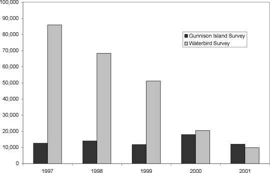
Snowy Plover

Peter Paton conducted an extensive ecological study of snowy plovers at GSL during the post-1980s high lake years and into the early 1990s (Paton 1994). This study followed Point Reyes Bird Observatory and the Utah Division of Wildlife Resources snowy plover inventories that suggested the snowy plover was prominent on the GSL landscape (Halpin and Paul 1989). Paton continued his snowy plover research in 1997 while under contract with the American Bird Conservatory. He carried out a replicate survey to those conducted in the early 1990s to see if the population had changed with any subsequent changes in the habitat. This survey overlapped the beginning year of the GSL Waterbird Survey. Paton’s survey team assisted in collecting all waterbird data for the Waterbird Survey in conjunction with surveying snowy plovers at the Locomotive Springs WMA.

Over seven years of surveying snowy plovers, Paton’s studies averaged 1121.8 plovers during peak periods. During the Waterbird Survey (1997-2001) peak counts for each year averaged 670.6. There were two exceptional count years in Paton’s study, 1991 and 92. These were transition years when extensive flats occurred that had once been occupied by emergent wetlands but were barren of vegetation as the GSL receded increasing extensive snowy plover and other shorebird habitat. If these two high count years are eliminated from the Paton sample, the difference between averages of Paton’s surveys and the Waterbird Survey is considerably less: 670 (Waterbird Survey) and 992 (Paton). The 1997 Paton and Waterbird Survey difference is very small, only nine percent, with numbers of 1,122 and 1,228 respectively (Table 14).

Beyond survey year differences, another influence in higher averages in the Paton sample is the conditions under which the information were collected. Paton et al developed a search gestalt only for snowy plovers. In contrast, Waterbird Survey volunteers were counting all waterbirds encountered. Under this system it becomes more difficult to pay the necessary attention to effectively search for the cryptic snowy plover. Given these conditions the peak counts are not out of line. Also, the survey routes for the Waterbird Survey stayed at 100 yard from the shoreline, and it is likely that in areas where the mudflats were extensive existing snowy plovers were too far from surveyors to be detected. The surveys in 1997 that overlapped may have been close in numbers because of the added emphasis on snowy plover detection by Paton’s surveyors who were rolling up their plover observations into the Waterbird Survey.

Table 14. Comparison of snowy plover data from the Waterbird Survey with Peter Paton studies.

Snowy Plovers
Year	1988	1989	1990	1991	1992	1993	1997	1998	1999	2000	2001
Paton Study (# of adults)	478	845	769	1344	1501	1150	1122	-	-	-	-
Waterbird Survey (# of adults)	-	-	-	-	-	-	1228	627	584	297	617

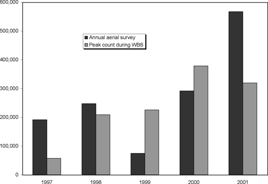
Wilson’s Phalarope

Wilson’s phalaropes present a survey challenge due to their use patterns of the GSL ecosystem. Starting in June they occur at GSL in large numbers and numbers build until they peak in July (Appendix 5, Wilson’s phalaropes). During this time, they aggregate into large flocks (tens to hundreds of thousands) that seem to develop patterns of occurrence that can change between years but remain somewhat constant within a year. These aggregations are usually birds standing on shorelines or in shallow water. During the day these large flocks break up into smaller foraging flocks (hundreds to thousands) that use the open water of GSL to forage brine shrimp and brine flies. They are often dynamic moving from one area of the lake to another. These conditions make surveying difficult from at least two perspectives. Sometimes the large flocks may be missed in aerial survey efforts to cover the 1,500 mi² lake and its vast associated shorelines. On the other hand small, mobile, open water foraging flocks are even more difficult to survey accurately because of their constant movements in and out of aerial survey transects. Wave action and cloud cover can exacerbate detection in open water environments.

Even so, there is a general trend shared by the two concurrent and independent surveys studying GSL Wilson’s phalarope: the WBS and a one-day aerial survey (Table 15 and Figure 11). One exception to the similar counts found by both surveys is the 1999 annual aerial survey. Here, two possible conditions may have occurred: the aerial survey missed one or more large aggregate flocks, or it missed the peak of migration. The five-year mean peak from the Waterbird Survey occurs during the second week of July. The annual aerial survey occurred on or close to July 29^th each year.

Phalaropes are dependent on the two major invertebrates that persist in the GSL when these birds are staging for migration to South America. Due to diluted brines at higher lake elevations and cool, wet weather 1998 and 1999 were years of low GSL macroinvertebrate production. Brine shrimp numbers were so low in Gilbert Bay that the brine shrimp harvest season was closed for that reach of the lake. The difference between the two surveys in 2001 is also interesting. During that year most of the Wilson’s phalaropes were located on the west shore near Carrington Island, outside of most Waterbird Survey areas.

Table 15. Comparison of Wilson’s phalarope data from the Waterbird Survey
with the annual aerial, all-lake, population count.

Wilson's Phalaropes
	1997	1998	1999	2000	2001
Annual aerial survey1	191,733	247,286	74,668	291,671	566,834
Waterbird Survey period 12 count2	57,328	17,431	81,478	25,021	242,344
Waterbird Survey peak count	57,328	208,461	225,488	378,292	318,974

¹ A one-day all lake survey conducted in late July each year.
² Period 12 includes the date of the annual one-day survey.

Figure 11. Graphical comparison of Wilson’s phalarope data from the
Waterbird Survey with the annual aerial, all-lake, population count.

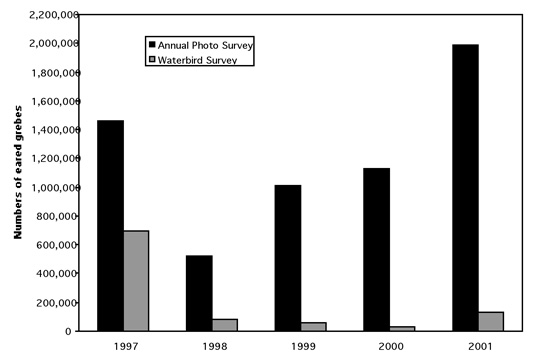
Eared Grebe

For a number of years, an annual eared grebe survey has been conducted during the molting period in October. This is a stratified photo survey that has been developed in cooperation with Hubbs Sea World Research Institute and the Canadian Wildlife Service (Boyd and Jehl 1998). Survey areas are georeferenced, flown by a series of transects, and photographed at intervals. The mean number of birds counted per unit area is used to extrapolate to the GSL population size. A portion of the fall eared grebe population falls within the GSL Waterbird Survey boundaries of Ogden and Farmington Bays, with another small proportion inhabiting the Bear River Bay system. However, the majority of the fall population occurs outside the Waterbird Survey boundaries in open lake water between Antelope and Stansbury Islands, around the Carrington and Hat Island complex, and extending up the west shore and north and west of Antelope and Fremont Islands. Because of this fact and the differences between survey techniques, comparisons between the two surveys are difficult (Table 16 and Figure 12). Also, the data from 1998 and 1999 reflect the absence of brine shrimp adults in the water column. This is important because when eared grebes are present at GSL, 99% of their diet is comprised of adult brine shrimp (UDWR unpublished data).

Table 16. Comparison of eared grebe data from the Waterbird Survey
with the annual population estimate using aerial photography.

Eared Grebes
	1997	1998	1999	2000	2001
Annual Photo survey1	1,460,151	522,287	1,008,656	1,127,307	1,987,564
Waterbird Survey	698,793	80,541	60,499	28,893	130,473

¹ Adjusted estimate. Survey conducted in mid-October of each year.

Figure 12. Graphical comparison of eared grebe data from the Waterbird Survey
with the annual population estimate using aerial photography.

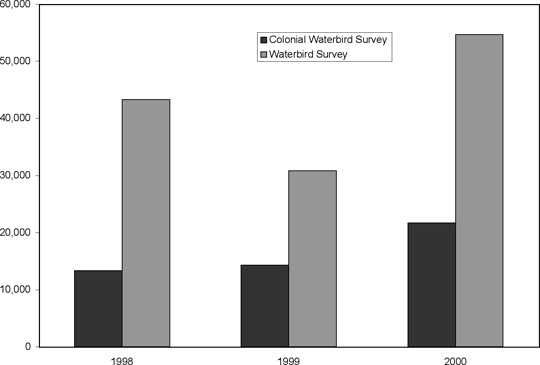
White-faced Ibis

Concurrent with the Waterbird Survey, colonial waterbird surveys were conducted for known colonies of species using emergent wetlands (Paul et al 2000b). This included white-faced ibises that often nest in conjunction with several other species. Franklin’s gulls, black-crowned night-herons, Forster’s terns, snowy egrets, cattle egrets, and a few others were frequently located together. The target of the colonial waterbird survey was to assess the number of breeding adults in the colony. The comparative Waterbird Survey data for the same years are uniformly higher and should be, as they include non-breeding adults, sub-adults, and hatching year birds in the count. However, the trends are similar between the two data sets (Table 17 and Figure 13).

Table 17. Comparison of white-faced ibis data from the Waterbird Survey
with the annual colonial waterbird breeding survey.

White-faced Ibises
	1997	1998	1999	2000	2001
Colonial Waterbird Survey	no count	13,294	14,260	21,664	1,896
Waterbird Survey peak count	47,577	43,265	30,779	54,634	34,854

Figure 13. Graphical comparison of white-faced ibis data from the Waterbird Survey
with the annual colonial waterbird breeding survey.

Management Implications

Implicit in the primary study objectives is the need to understand species habitat relationships for more effective management and stewardship. Many of the data analyses, if not all, were developed and executed to assist local resource managers in making wise and cogent decisions for a long term, sustainable GSL ecosystem. This study, basically a systematic inventory, and its database were used to gather and store data from which specific questions can be queried. Through some analyses, we have answered questions that will assist managers and decision makers as they seek to protect and conserve GSL resources. Some of these analyses follow.

Georeferenced Survey Areas

At the onset of the study, survey areas were delineated in discrete units with physical descriptions. These areas were placed into logical blocks that comprised similar resource areas (i.e., WMAs, stretches of shoreline, open water, islands, etc.). Later the database manger, with the assistance of Dave Mann and other UDWR GIS (Geographic Information Systems) staff georeferenced each survey area. Then, survey areas where sampling was conducted were further refined to a percent of the area that was actually covered by survey effort. This process allowed for inter-area contrast through the application of population and species density comparisons (Appendix 4). Geographically referenced sites also allow resource managers to combine adjoining sites, or even similar habitat types that are not joined for evaluation. This can be either a quantitative or qualitative tool for comparative analyses on prioritizing conservation actions.

Survey Area Descriptions

Survey Area Descriptions may be the single most important source of information to evaluate on-the-ground bird presence in specific locations (Appendix 4). This is the density information by species. These data should be used with the knowledge that since it is an average of 77 surveys over five years, a five-year mean is a strong number with considerable comparative value. These years represent a good variation of wet and dry conditions, and reflect past times of lake fluctuation of five feet in elevation. On the other hand, the extreme situations are tempered in mean data, and therefore, it is of value to examine individual years and survey periods to get a clearer picture of what might happen under specific circumstances. There are times in a survey area when a species or suite is notably present, without an understanding of why that is the case.

Other information that may be of import to resource managers is species diversity. In this report, species diversity is defined as the number of species occurring in an area in high presence values. These individual area accounts will provide information on coverage by year and some comments on survey detection rates.

Species Accounts

This report presents Species Accounts for the majority of species identified during the Waterbird Survey (Appendix 5). Due to small data size or irregular occurrence, however, there are some species excluded. The information is presented in order to help resource managers grasp the importance of the GSL population compared to the North American and/or global populations where numbers were available. A graph of the mean five-year counts by survey period provides information on seasonal presence. Perhaps of greatest value in importance assessment for habitat use is in the species distribution plots georeferenced to a GSL map. This map reflects an over all area habitat use value of the five-year mean. This might be the answer to general questions like “which area(s) is most important for American white pelicans.” The answer from the map is the Bear River Bay complex, and is true if you roll all survey periods into one mean; but without Gunnison Island (the breeding colony) for a substantial number of these pelicans using the Bear River system, this map would be altered significantly. To assist in the evaluation of areas important to species use at GSL, it will be important to inspect the specific Survey Area Descriptions (Appendix 4) and to consult the Species Distribution by Survey Period section (Appendix 6). These analyses and others in the report will help develop a more precise picture of bird use of the GSL.

The pelican example brings to light the observation that breeding populations in the area sometimes influence the Waterbird Survey data for specific areas, regions and populations of the lake. Breeding populations were not accounted for in this study. The only time breeding populations are considered is in some of the narrative of specific Survey Area Descriptions. Yet, colonial nesting populations and loosely associated nesters (i.e., American avocets were frequently associated with survey areas and routes) did influence counts in many areas. There was no attempt to avoid them; they were counted uniformly across the landscape along with non-breeding populations.

Species Distribution by Survey Period

Information important during different periods of the survey season is available here. This information represents a five-year mean for each survey period (1-17). These temporal data are important to evaluating seasonal use of each species. Cinnamon teal distributions through time is prominent in the Bear River Bay during the early to mid survey periods (April-July), and becomes equally or more important in the Ogden and Farmington Bay WMAs at the end of the season (August-September).

The vast majority of marbled godwits are located in the Bear River Bay system through both the spring and late summer use periods. Managers considering the GSL’s role in godwit conservation need to pay close attention to the Bear River MBR and the Willard Spur systems. Why birds occur at certain times in specific places is a question not answered for most species in this study.

Migration Chronology

This report provides a migration chronology similar to the information on presence status in Birds of Utah (Behle and Perry 1975), but refined for GSL (Table 6). Habitat managers and biologists are often requested to provide recommended windows of time for development or potential disturbance activities. These “best time, worst time” requests are difficult without systematically collected temporal data. Therefore, this migration chronology should assist resource mangers in designing best-case scenarios.

Shoreline Conservation

The numerous shoreline survey area data sets confirm the critical role that GSL shorelines habitats play for a variety of species for most phylogenetic groups in the GSL ecosystem. Several of the analyses provided in the report can assist in the understanding of shoreline habitat characteristics and values.

Point sample data are the only information describing habitat use by waterbirds in the study. These data are summarized for the high lake study year, 1999, and the low lake year, 2001, only. Mean bird counts are compared by suite, habitat type, and year. Charts compare mean bird counts for all habitat types combined for 1999 and 2001. Due to the dynamic condition of the shoreline, which is an important value and phenomenon in lake avian ecology, this information should be used to predict bird use at different elevations and for developing shoreline management strategies. The data collected in this study makes clear the critical role shoreline fluctuations play in bird and wetland succession. For this reason, shorelines should be allowed to expand and contract through their full range with minimal anthropogenic developments.

When point samples were established at GSL in 1997, certain randomly selected points were put in place to compare with bird use data collected from non-drainage points. The comparison between these two point sample types is difficult because we do not have good flow rates at drainage points. Some were established where irrigation returns enter the GSL; flow regimes are difficult to measure at these sites due to the intermittent flows associated with agriculture water systems. In some cases drainages were discontinued altogether, and the drainage point sample became a non-drainage point in terms of presence of water and bird use.

Managed Wetlands

Until this study, there had not been an effort to collect coordinated data between wetland managers (State, Federal and non-profit). With this study, wetland managers will be able to determine which species and for which time of year their management areas are important. The data will also make coordinated conservation actions between management areas a more viable possibility. These data provide some information on species values by area that can assist managers in developing management practices that best suit their areas and intrinsic habitat values.

In addition to total count data, most State managers incorporated area counts into their sampling program during the study. These area counts were conducted in defined sites, bounded by dikes or other borders, that have or could be georeferenced to compute density data for comparison. The area counts assess the area in the same way that occurred in point samples. Area counts were suggested as a tool for managers to use in assessing treatment values to the area. These could include controlled burns, drawdowns and flooding, and chemical treatments. The study allowed the managers to choose area count sites within their sampling scheme. This approach was developed for managers to use as a tool and not as an element to be analyzed in this report. Data were provided annually to managers for their use. The use of this technique can be applied in time and is suggested as a possible evaluation tool for future treatments.

The data sets for managed areas are among the richest in species composition and numbers of birds that occurred in the five-year study. The individual and collective data sets for emergent vegetation survey areas, the species accounts, and chronological bird data are some useful tools to consider for managers.

The Great Salt Lake

Bird use of the GSL is substantial but varies by area, time of year, and lake elevation. The three open lake regions of the GSL that were surveyed, Farmington Bay, Ogden Bay, and Bear River Bay, each offer significant avian values. Managers can assess the values by examining the individual Survey Area Descriptions (Appendix 4).

Managers should carefully consider shoreline associations of each of these lake regions. Lake elevation should also be considered when evaluating annual data. Most of the data are represented as a five-year mean, but there is a sample of high and low lake elevation, 1999 and 2001 respectively, in the Appendix 8. There is also a high and low lake year data set for GSL shoreline use as described through point sample data (Appendix 3).

Important to the Farmington Bay region is the occurrence of large sandbars in the south part of the bay between the mainland and the southeastern portion of Antelope Island and south of the Great Salt Lake Shorelands Preserve. These formations are two of the most dynamic features at GSL. Carefully consider bird data in this area by lake elevation. An interesting pattern of bird use occurs at different lake elevations in the Layton Wetland complex as well.

Within the study area, East Gilbert Bay is the primary producer of brine shrimp and is an extension of the main Gilbert Bay where the vast majority of brine shrimp are produced. This area is also affected by lake elevation, but not in the same way as Farmington Bay. Here, WMA dikes at Howard Slough and Ogden Bay are submerged when GSL is above 4202' ASL. Managers should pay attention to lake elevation and brine shrimp and fly production when evaluating bird data in this area. These is no current brine fly monitoring at GSL, but the Great Salt Lake Ecosystem Project files have good brine shrimp harvest and density data since 1996. Great Salt Lake elevation records generally correlate to brine densities, and these data are available through Utah Geologic Survey, Utah Department of Natural Resources.

The Bear River Bay region is an intermittent fishery and the associated waterbird presence is profoundly influenced by the fishery condition. The most extensive wetlands occurring outside management areas occur here. When there are low flows in the Bear River and the GSL is at 4200' ASL or below, the fishery in the Bear River Bay and Willard Spur is dysfunctional. When flows are average or greater and elevations are at 4202' ASL or higher, there is a consequential fishery and piscivorous bird presence in the area. The difference can be tens of thousands of birds. During the dry climate condition, much of the outlying emergent wetlands are dry. During wet cycles robust emergent waterbird colonies are present; some colonies are the largest in western North America. These are especially important to white-faced ibises and Franklin’s gulls. Here again five-year mean data are of value but particular attention should be paid to individual year records measured against Bear River flows and lake elevation.

Habitat and Population Modeling

Some modeling of habitat and potential species presence exists using the database and this report. Because this study was an ecosystem based systematic survey that covered all prominent habitats, modeling is a real possibility. This survey can be used to refine the model that is currently in place to assess brine shrimp harvest impacts on avian resources.

Conservation Planning

This data set and subsequent report provide a foundation of biological and habitat information for conservation planning within the ecosystem. The surveys took place over several years and during five feet of vertical lake elevation change, and provide a reasonable picture of how the lake is used by waterbirds under a variety conditions, and through much of recorded lake elevation history. However, it is important to remember that extreme events did not occur during this survey. Extreme events (i.e., historic lows and highs) can have dramatic effects on wildlife populations and their habitats.

This information will also be useful in evaluating existing plans such as the GSL DNR Comprehensive Plan, regional and national shorebird and waterbird plans, and Intermountain West Joint Venture Focus Area plans. The draft GSL Shorebird Plan will perhaps benefit the most from this data set as it validates assumptions and offers new information. The GSL Waterbird Survey Report will be helpful in defending the 23-21-5 designation authorized by the Utah state legislature that allows for wildlife management primacy in several sections of State land within Farmington, Bear River, Gilbert and Gunnison Bays.

The information collected in this study is already being utilized with the Western Shorebird Survey. This survey is a subset of data being collected to monitor national and continental shorebird populations. Utah was one of the first states to come on line in the Western Shorebird Survey with survey sites, surveyors and data sets already in place. This web-based approach to data collection is unique in the western shorebird monitoring community.

This study with its impressive bird numbers and demonstrative species value should be used to emphasize the importance of the system to communities and their leaders. Bird use days, peak populations and the strength of the five-year mean data are selling points from Syracuse, Utah to Washington D.C. These data validate the anecdotal observations and less robust data sets by describing in more detail, with greater accuracy and more reliable data, the value of the GSL in the Western Hemisphere setting. This story should be told.

Go to Previous Section (Habitat Use) • Go to Next Section (Recommendations)...